TPDstat Cheat Sheet

library(tidyverse)
library(gov50data)

R Basics (Week 1)

Creating a vector

You can create a vector using the c function:

## Any R code that begins with the # character is a comment
## Comments are ignored by R

my_numbers <- c(4, 8, 15, 16, 23, 42) # Anything after # is also a
# comment
my_numbers

[1]  4  8 15 16 23 42

Installing and loading a package

You can install a package with the install.packages function, passing the name of the package to be installed as a string (that is, in quotes):

install.packages("ggplot2")

You can load a package into the R environment by calling library() with the name of package without quotes. You should only have one package per library call.

library(ggplot2)

Calling functions from specific packages

We can also use the mypackage:: prefix to access package functions without loading:

knitr::kable(head(mtcars))

	mpg	cyl	disp	hp	drat	wt	qsec	vs	am	gear	carb
Mazda RX4	21.0	6	160	110	3.90	2.620	16.46	0	1	4	4
Mazda RX4 Wag	21.0	6	160	110	3.90	2.875	17.02	0	1	4	4
Datsun 710	22.8	4	108	93	3.85	2.320	18.61	1	1	4	1
Hornet 4 Drive	21.4	6	258	110	3.08	3.215	19.44	1	0	3	1
Hornet Sportabout	18.7	8	360	175	3.15	3.440	17.02	0	0	3	2
Valiant	18.1	6	225	105	2.76	3.460	20.22	1	0	3	1

Data Visualization (week 1)

Scatter plot

You can produce a scatter plot with using the x and y aesthetics along with the geom_point() function.

ggplot(data = midwest,
       mapping = aes(x = popdensity,
                     y = percbelowpoverty)) +
  geom_point()

Smoothed curves

You can add a smoothed curve that summarizes the relationship between two variables with the geom_smooth() function. By default, it uses a loess smoother to estimated the conditional mean of the y-axis variable as a function of the x-axis variable.

ggplot(data = midwest,
       mapping = aes(x = popdensity,
                     y = percbelowpoverty)) +
  geom_point() + geom_smooth()

`geom_smooth()` using method = 'loess' and formula = 'y ~ x'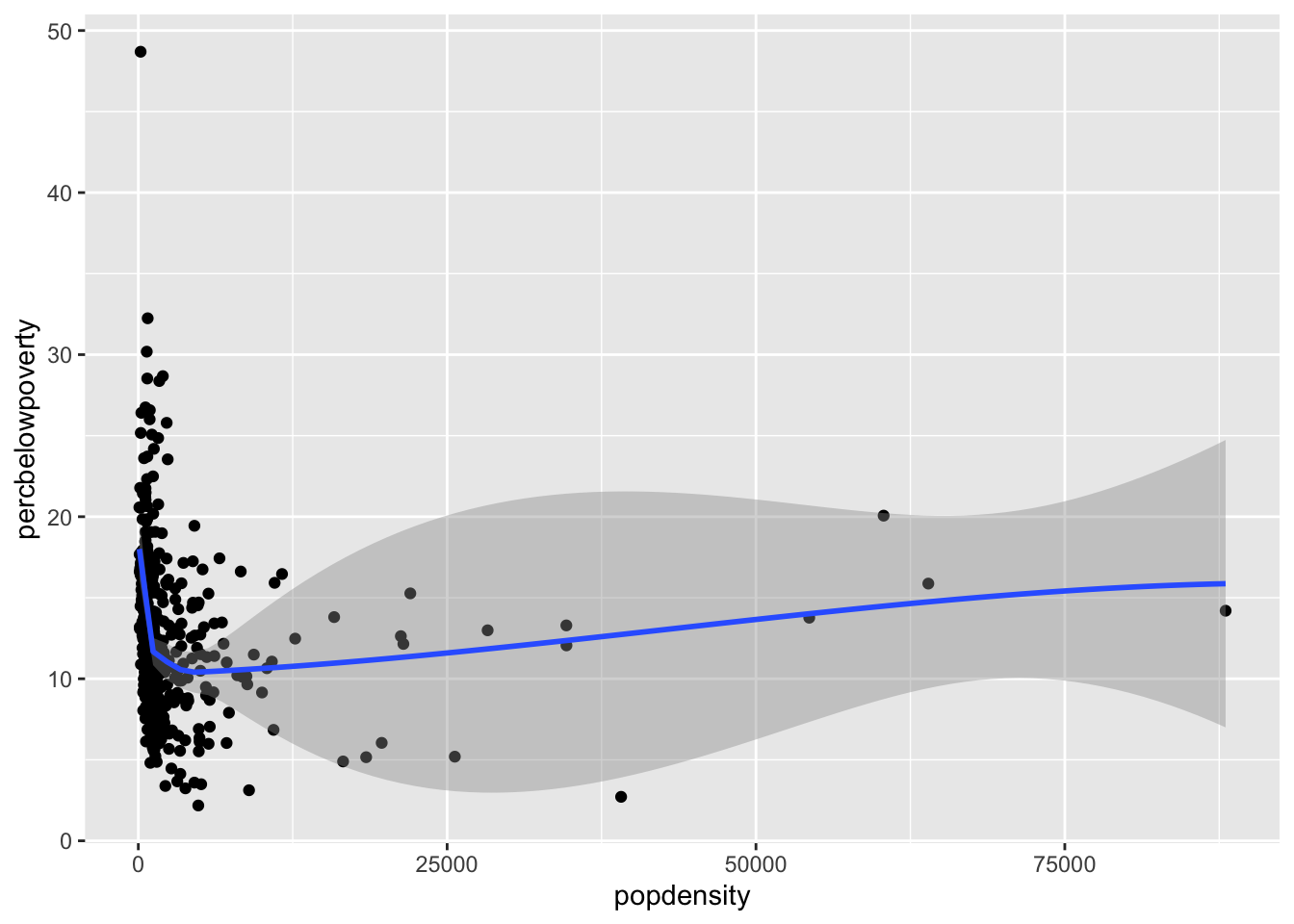

Adding a regression line

geom_smooth can also add a regression line by setting the argument method = "lm" and we can turn off the shaded regions around the line with se = FALSE

ggplot(data = midwest,
       mapping = aes(x = popdensity,
                     y = percbelowpoverty)) +
  geom_point() + geom_smooth(method = "lm", se = FALSE)

`geom_smooth()` using formula = 'y ~ x'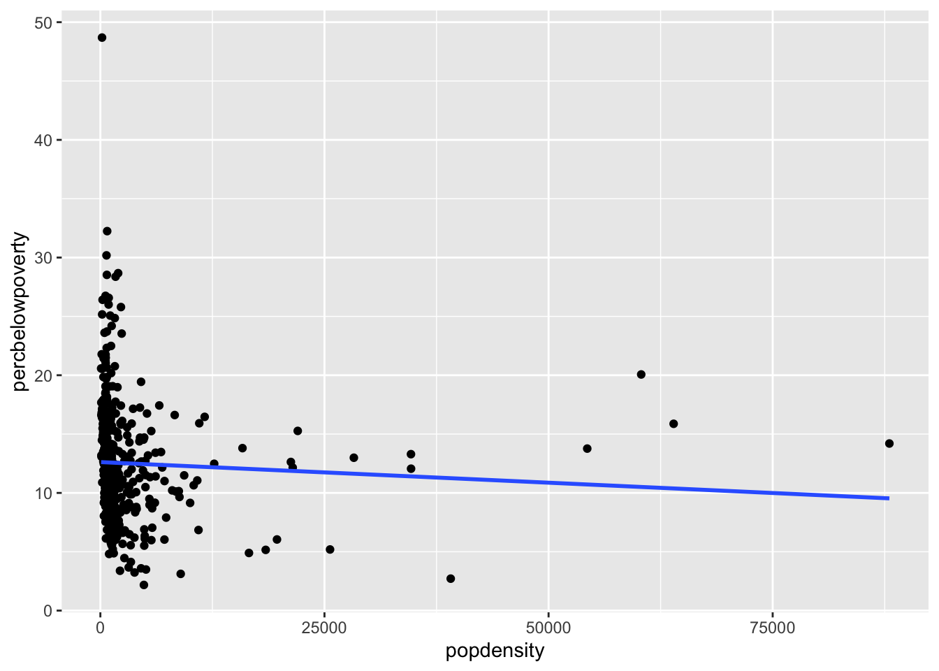

Changing the scale of the axes

If we want the scale of the x-axis to be logged to stretch out the data we can use the scale_x_log10():

ggplot(data = midwest,
       mapping = aes(x = popdensity,
                     y = percbelowpoverty)) +
  geom_point() +
  geom_smooth(method = "lm", se = FALSE) +
  scale_x_log10()

`geom_smooth()` using formula = 'y ~ x'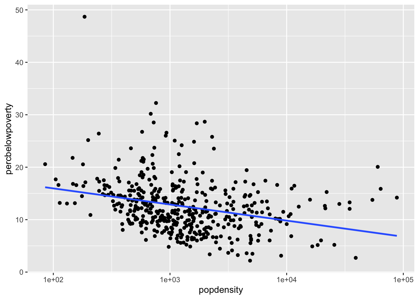

Adding informative labels to a plot

Use the labs() to add informative labels to the plot:

ggplot(data = midwest,
       mapping = aes(x = popdensity,
                     y = percbelowpoverty)) +
  geom_point() +
  geom_smooth(method = "loess", se = FALSE) +
  scale_x_log10() +
  labs(x = "Population Density",
       y = "Percent of County Below Poverty Line",
       title = "Poverty and Population Density",
       subtitle = "Among Counties in the Midwest",
       source = "US Census, 2000")

`geom_smooth()` using formula = 'y ~ x'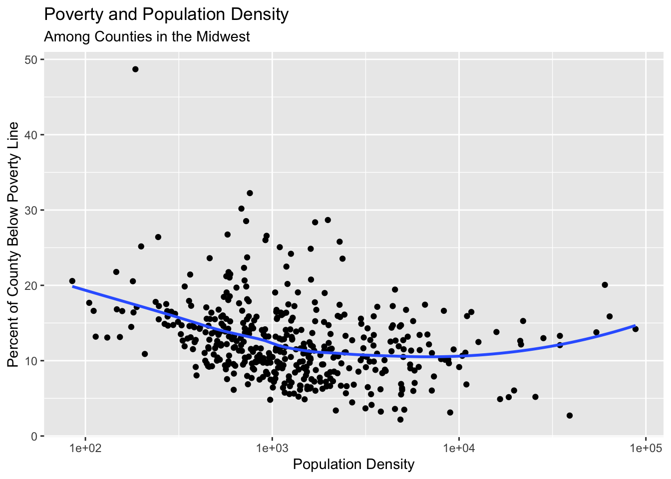

Mapping aesthetics to variables

If you would like to map an aesthetic to a variable for all geoms in the plot, you can put it in the aes call in the ggplot() function:

ggplot(data = midwest,
       mapping = aes(x = popdensity,
                     y = percbelowpoverty,
                     color = state,
                     fill = state)) +
  geom_point() +
  geom_smooth() +
  scale_x_log10()

`geom_smooth()` using method = 'loess' and formula = 'y ~ x'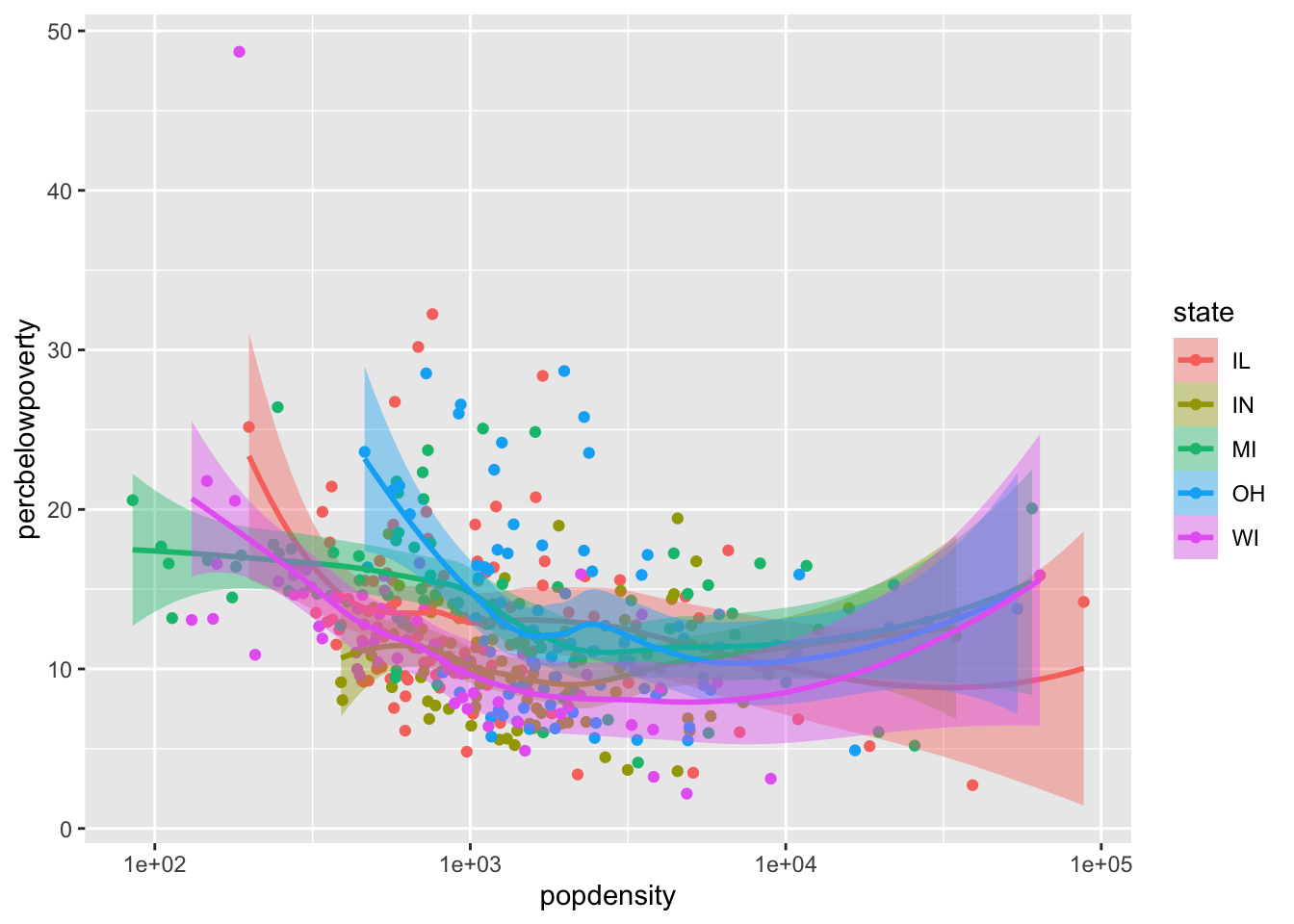

Mapping aesthetics for a single geom

You can also map aesthetics for a specific geom using the mapping argument to that function:

ggplot(data = midwest,
       mapping = aes(x = popdensity,
                     y = percbelowpoverty)) +
  geom_point(mapping = aes(color = state)) +
  geom_smooth(color = "black") +
  scale_x_log10()

`geom_smooth()` using method = 'loess' and formula = 'y ~ x'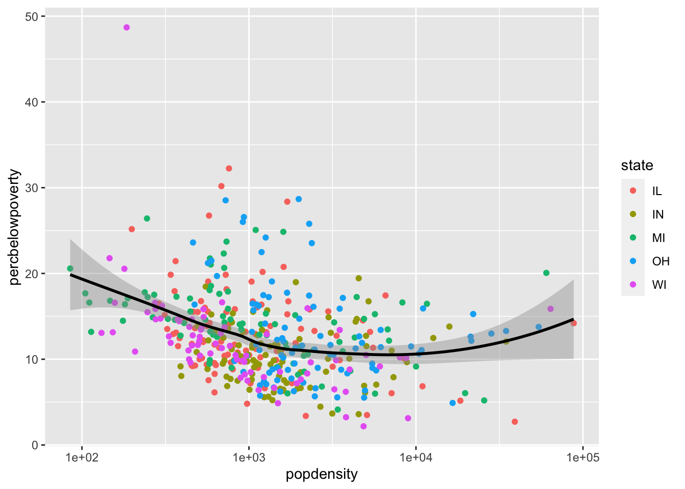

Setting the aesthetics for all observations

If you would like to set the color or size or shape of a geom for all data points (that is, not mapped to any variables), be sure to set these outside of aes():

ggplot(data = midwest,
       mapping = aes(x = popdensity,
                     y = percbelowpoverty)) +
  geom_point(color = "purple") +
  geom_smooth() +
  scale_x_log10()

`geom_smooth()` using method = 'loess' and formula = 'y ~ x'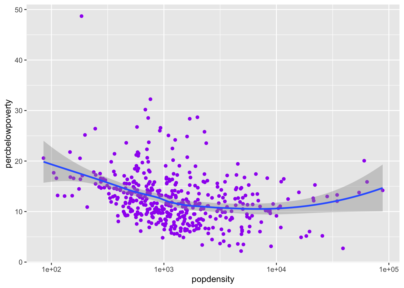

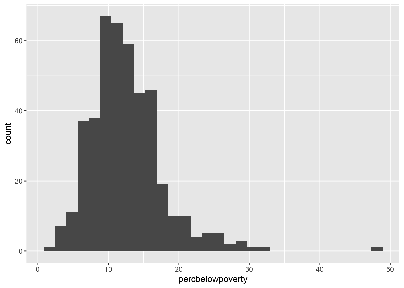
Histograms

ggplot(data = midwest,
       mapping = aes(x = percbelowpoverty)) +
  geom_histogram()

`stat_bin()` using `bins = 30`. Pick better value with `binwidth`.